R from gvSIG perspective
An introduction to gvSIG geoprocessing
Geostat course, Albacete 2016
Cesar Martinez Izquierdo - www.scolab.es
Contents
- Workshop goals
- Software installation
- Introduction to gvSIG
- Interacting with R
- Exercises
Workshop goals
- Get an overview of gvSIG, a full featured desktop GIS software
- Learning about how to use R from gvSIG
- Demonstrate gvSIG geoprocessing and visualization capabilities, using a case study
Software installation
The following software is required for the course:
- gvSIG 2.3.0 rc4 (or later)
- gvSIG-Rexternal (gvSIG plugin)
- R statistical software
Press Down key for details
gvSIG 2.3.0 rc4 (or later)
- Get the software from the Development versions download section at gvsig.com
- The installable version is recommended
- But you can also use the portable version (no installation required)
- If using Linux, choose the gvSIG version suitable for your Linux version (e.g. Ubuntu 16.04 vs 14.04)
R statistical software
Download and install from CRAN
gvSIG-Rexternal (gvSIG plugin)
- Download from the dist folder of the plugin Github repo. You need the last available .gvspkg file (version 1.0.2-6 as of October 2016)
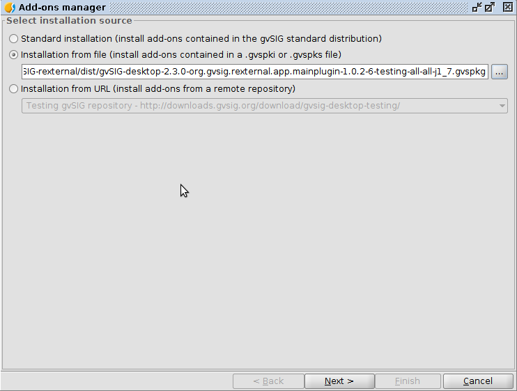
- Install using gvSIG Add-ons manager (Menu: Tools -> Add-ons manager)
- Choose Installation from file to install the downloaded .gvspkg file
- Select Rexternal from the list of available plugins
- Note that you may need to execute gvSIG as Administrator in order to install plugins in Windows
gvSIG-Rexternal (gvSIG plugin)
gvSIG-Rexternal (gvSIG plugin)

gvSIG-Rexternal (II)
Test that RExternal is correctly installed by launching RShell using the gvSIG Scripting launcher

gvSIG-Rexternal (III)
It should open a new R console
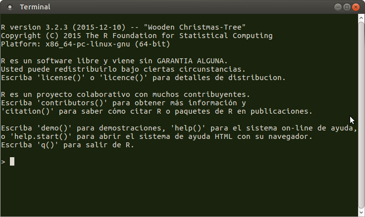
Check the next slide if you find any problem
gvSIG-Rexternal (IV)
- RExternal tries to guess the R installation folder, but you may need to manually configure it
- If needed, edit the file
gvSIG/extensiones/org.gvsig.rexternal.app.mainplugin/rpath.propertieswithin your gvSIG installation folder - You need to write the full path to the R executable, as shown in the examples
# File: gvSIG/extensiones/org.gvsig.rexternal.app.mainplugin/rpath.properties
# keep this empty to search R binary in current PATH
R_BIN_PATH=

## You can manually set the path to the R binary. Examples:
#
# Typical path for Linux:
# R_BIN_PATH=/usr/bin/R
# Typical path for Windows 64 bits:
# R_BIN_PATH=c:\\Program Files\\R\\R-3.2.3\\bin\\x64\\R.exe
# Typical path for Windows 32 bits:
# R_BIN_PATH=c:\\Program Files\\R\\R-3.2.3\\bin\\x32\\R.exe

## Note that in Windows, the path to R will likely change when
## you update R to a newer version!!!!!

## You can also use an internally-installed R instance
# R_BIN_PATH=R/bin/R
Install extra symbol libraries (gvSIG plugins)
- Install using gvSIG Add-ons manager (Menu: Tools -> Add-ons manager)
- Choose Standard installation
- Install all the available symbol libraries
- Note that you may need to execute gvSIG as Administrator in order to install plugins in Windows
R packages
Install the following R packages: rgdal, sp and raster.
Type in R console:
install.packages("sp")
install.packages("raster")
install.packages("rgdal")
Introduction to gvSIG
- Overview
- Vector layers
- Raster layers
- Remote services
- 3D views
- Geoprocessing
- Scripting
Overview
- gvSIG is a desktop geographic information system (GIS) application
- Available for Linux, Windows and Mac
- Translated to 18 languages
- Long history: first version released on 2004
- GPL3 license
Overview (II)
- Vector and raster data support
- Support for data bases, remote services (OGC's WMS, WMTS, WFS, WCS, etc) and other tile providers (OSM/Map Quest, Google, etc)
- Vector editing capabilities
- 3D visualization
- Map composer
Overview (III)
- Geoprocessing tools and process modeller
- Easily extensible using the integrated scripting framework and the Add-on manager
- Different scripting languages supported (Python/Jython, Groovy, R/Renjin, Javascript and Scala)
gvSIG documents
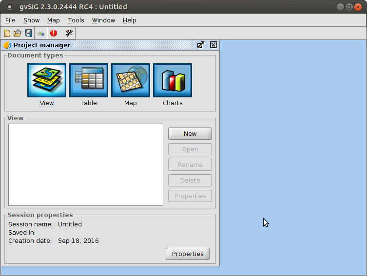
gvSIG documents
- Views: data visualization, processing and editing
- Table: alphanumeric information visualization/editing
- Map: map composition, printing and high quality exporting
- Charts: create simple charts
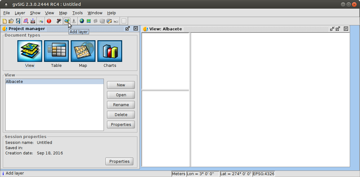
Views: Add layer
Vector data
- Advanced symbology and labelling
- Lots of formats supported: SHP, PostGIS, DXF, DGN, GML, KML, LAS (LIDAR), CSV and Excel points...
- Plus all the formats supported by OGR
Add layer: files

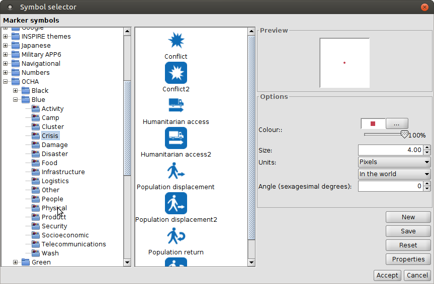
Symbol library
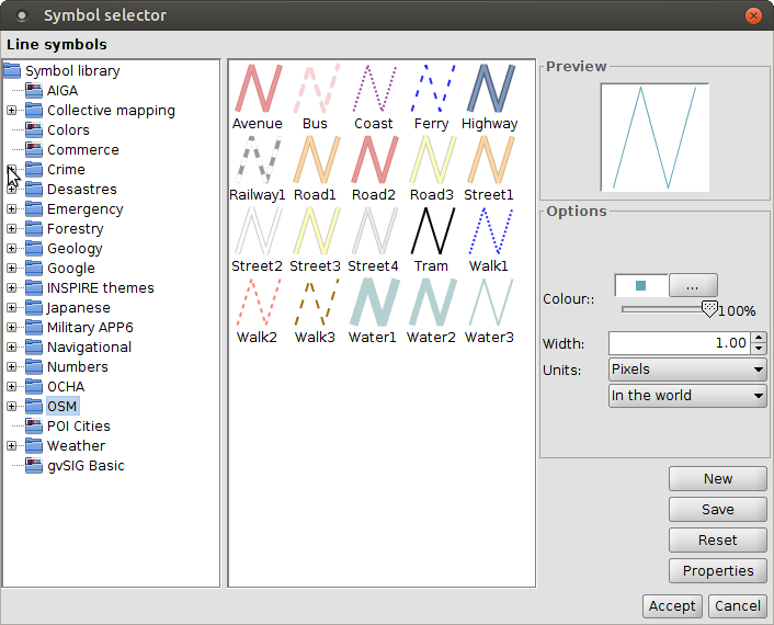
Symbol library
Raster data
- Uses GDAL to read most formats
- Analysis view, colour tables, histograms, etc
WMTS layers
3D views
- Creates 3D views from 2D views (layers, symbology, etc)
- Viewport and layer synchronization between views
- Spheric and flat modes
- Anaglyph mode
3D views: LIDAR data
3D views: vector extrusion
Geoprocessing
Geprocessing
- Raster and vector processing tools
- 355 tools available (including Sextante)
- General purpose and specific (hydrology, forestry, etc) tools
- More tools available as plugins: JGrass tools (forestry, LIDAR, hydrology...)
- Creation of new tools is simple (Python, Java, R...)
Process modeller
Process modeller
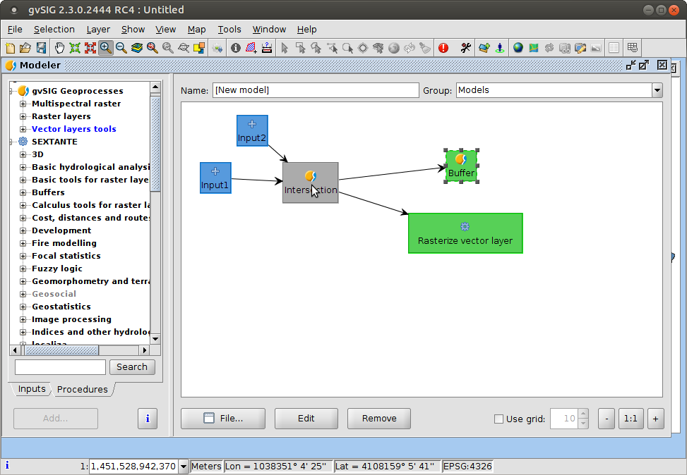
Process modeller
- Simple while powerful tool to define models or automating processing flows
- Useful for streamlining complex analysis
Scripting framework
- Useful for extending gvSIG or automate tasks
- Allows to create:
- new buttons, menu entries, forms
- new geoprocessing tools (and use them in the modeller)
- Integrated scripting composer and launcher
- Integrated console (Python)
- Simplifies creation of new gvSIG plugins
Scripting framework
Interacting with R
- Two different R plugins (and approaches) in gvSIG:
- Renjin (Java based R implementation)
- RExternal plugin (uses an external R process)
- They offer totally different possibilities and limitations
Renjin
- Integrated in the gvSIG Scripting framework
- Makes possible to control or automate gvSIG from an R script (layer loading, accessing to layer values, etc)
- Limitations:
- Only a small fraction of the existing R packages are available on Renjin
- For the moment, no direct way to load R data frames as gvSIG tables or accessing gvSIG tables as R data frames
Renjin
- Installation of packages works in a different way, compared to the regular R implementation
- Packages get automatically installed when the library() command is used
- The availability of each package for Renjin can be checked on this page
RExternal plugin
- Allows to launch R scripts from gvSIG
- Runs as an external R native process (so any R package can be used)
- Provides an easy way to pass gvSIG layers as inputs to the R script and to load R outputs as gvSIG layers
- R scripts can be registered as gvSIG Geoprocesses and included in gvSIG models
RExternal plugin
- Limitations:
- Requires a small script declaration (written in Python) per each R script
- Data interchange is limited to input/output layers/tables
RExternal plugin
- The integrated R script can be very easily packaged and distributed as gvSIG plugin
- The user interface for the process is automatically built (based on the declaration of parameters)
RExternal plugin
RExternal plugin

RExternal plugin
See Exercise 3 for detailed documentation and usage examples
Exercises
Download and uncompress the sample data and sample scripts for the exercises
Exercise 1
Goal: getting familiar with gvSIG basics
Exercise 1: Views and data
- Create a new view: Project Manager -> View -> New
- Change some View properties:
Exercise 1: Views and data
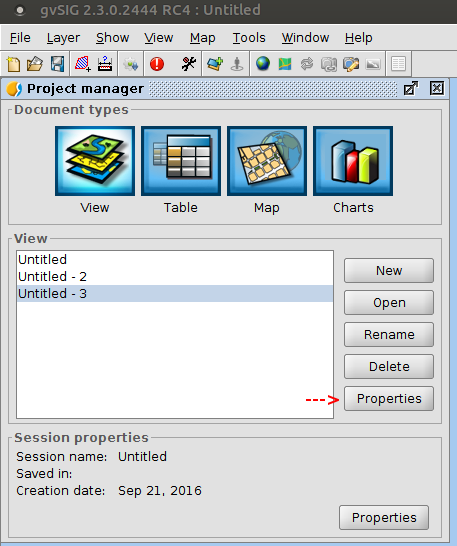
Exercise 1: Views and data
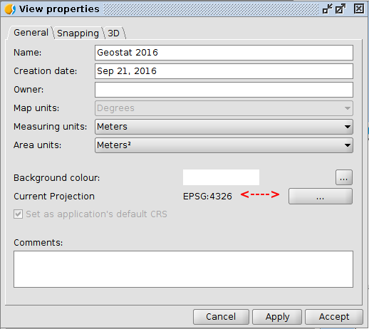
- Change some View properties:
- Set a meaningful name: Spain
- Configure a proper reference system for the view. We'll work with Spain data, so we'll use UTM zone 30N with ETRS89 datum (code EPSG:25830)
- It is important to set the CRS before loading any layer
Exercise 1: Views and data
Exercise 1: Views and data
- Load some vector layers
Exercise 1: Views and data
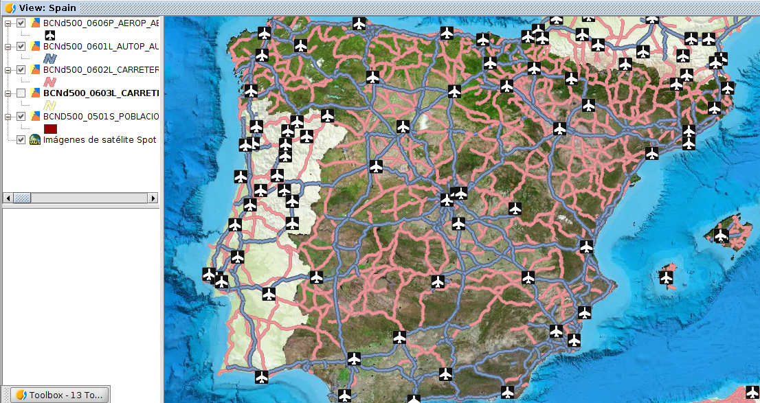
- Load all the layers under the bcn500_cnig folder
- They contain information about:
- Points: airports
- Lines: motorways, primary and secondary roads
- Polygons: main agglomerations
Exercise 1: Views and data
- Apply proper symbology to each layers (select layer in TOC & then double click on it)
- You can define your own symbology or use the symbol library
- Suggestion: use OSM symbols for roads and airports
Exercise 1: Views and data
- You can load an online satellite image as background
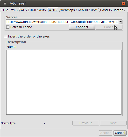
- Go to Add layer -> WMTS
- Use service
http://www.ign.es/wmts/pnoa-ma?request=GetCapabilities&service=WMTS - Connect to the service and follow the wizard
- Choose the proper reference system (EPSG:25830)
Exercise 1: Views and data
- Reorder the layers on TOC:
- move the satellite image and the polygon layer to the bottom
- move the airport layer to the top
- order the roads by importance
- You can also set the secondary roads layer to be only visible at a certain scale (on layer properties)
Exercise 1: Views and data
Exercise 1: Views and data
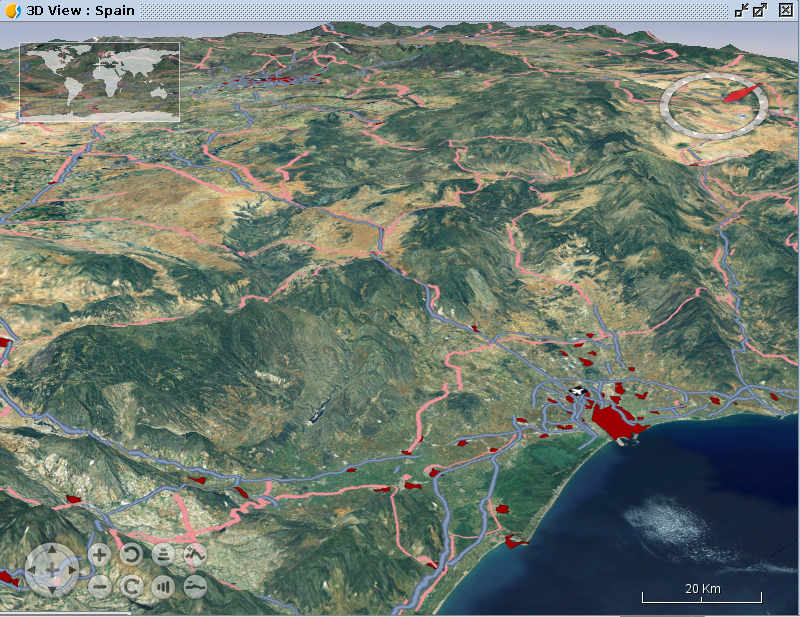
- Create a 3D spheric view
- Use terrain exaggeration to make it more impressive
- Hints:
- You can use the mouse and shift keys to navigate faster
- You'll see a reprojection artifact in the WMTS layer. You can disable it (as there is a built-in satellite image on the 3D view) or create the 2D view using EPSG:4326 to avoid this artifact
- Use the Animation manager to create a visualization
Exercise 1: Views and data
- Use the Animation manager to create a visualization
- Set at least 5 animation steps
Exercise 1: Views and data
Exercise 2
Goal: Demonstrate the geoprocessing toolbox
Exercise 2
We have some information about species distribution (from the SPANISH INVENTORY OF TERRESTRIAL SPECIES) and want to learn about the habitat preferences of a particular species (Otis tarda).
We also have information about land cover and elevation
Hi, I am Otis tarda!!
Image: Francesco Veronesi (CC BY-SA 2.0)
I am also Otis tarda
Image: Governor of Volgograd Oblast (CC BY-SA 3.0)
Exercise 2
- First, we need to load the species distribution information
- We have a shapefile defining a reference grid and a CSV that defines in which cells of the grid the species is present
- Load the layer Malla10x10_MarTierra_p.shp
- Go to Project Manager and create a new table to load the CSV (otis_tarda_latin1.csv or (otis_tarda_utf8.csv)
- Hints:
- When loading the table, go to properties and select Profile: Excel
- Use the latin1 csv in Windows and utf8 otherwise
- Or choose the proper encoding in advanced properties tab
Exercise 2
- Now we need to relate the shp with the csv information, using the Join tool
- From the newly created table, go to menu Table -> Create join
- Choose the SHP as the first data store to join, the csv as the second one
- The fields containing the related keys are CUARDICULA and CUTM10X10.
- We'll only need the Grupo, Nombre, Genero and Especie fields from the CSV
Exercise 2
- Now we want to select only the cells with species presence
- On the joined layer, use tool Select By Attribute (menu: Selection)
- Select the records having Otis tarda as name, creating a new selection set
Exercise 2
- Now we'll export the selected cells to a new layer
- From the view TOC, right click on the joined layer and select Export to...
- Export to a new SHP, including only selected records
- Performance tip: do some cleaning, hide or remove all the previous layers
Exercise 2
- Now we want to know in which types of land cover the species can be found
- We'll cross the information and get some statistics
Exercise 2
- Load clc2006_250 raster layer, containing land cover information for the year 2016 from the European dataset Corine Land Cover
- There are two equivalent class codes
- The one used in the raster file (from 1 to 44)
- A hierarchical code (1, 1.1, 1.1.1, 1.1.2, 2, 2.1, etc)
- There is a txt file next to the layer, providing information about the class definitions and code equivalences
Exercise 2
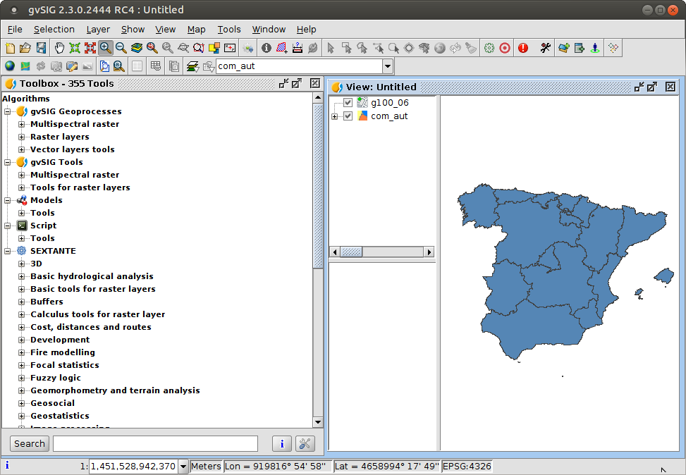
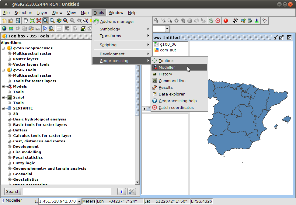
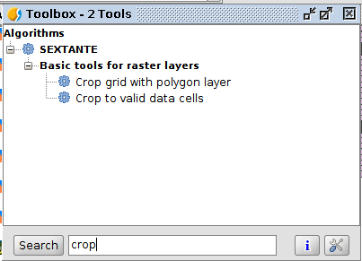
- Open the Geoprocessing toolbox (menu: Tools: Geoprocessing: Toolbox)
- There is a large list of processes available
- You can filter them using the search box (down)
- Some of them are disabled because there is no suitable input layer for them in the view
Exercise 2
Exercise 2
- Use the Crop grid with polygon layer algorithm to extract the land cover classes that overlap with the species presence areas
- Then use the Class statistics algorithm to get the frequency of each land cover class in the presence areas
- Hint: The output of the Class statistics algorithm is a table, you can open it from the Project Manager
Exercise 2

Exercise 2
- Now you can use the elevation data for performing a similar analysis
- Load the elevation data (ign_mdt200)
- Use the Geoprocessing Toolbox to calculate the slope from the elevation (as slope usually influences species habitats)
- Think yourself about an appropriate methodology to analyse this information
Exercise 3
Goal: Demonstrate the gvSIG-R interface using RExternal plugin
Exercise 3
We are going to learn how to integrate R scripts in the gvSIG Geoprocessing Toolbox and how to easily distribute them as new gvSIG plugins
Exercise 3
- First we'll study the structure and code of the provided sample plugins.
Start by looking at the
geostatspluginfolder. We'll have 4 components: - The R script we want to integrate
- A bit of Python glue-code to declare the R script parameters and methods
- An small
autorun.pyscript to register the script in the Toolbox - An empty
__init__.pyfile - There is also some .inf files but they are automatically created by gvSIG when the scripts are created
Exercise 3
Have a closer look to each file. In test.r script we have: 1) a function to load some
libraries:
load_libraries <- function() {
  library(rgdal)
  library(raster)
  return(1)
}
Exercise 3
Have a closer look to each file. In test.r script we have: 2) a doalmostnothing function
which loads a vector layer and copies one raster from inrasterpathname to outrasterpathname:
doalmostnothing <- function(shpdsn, shpname, inrasterpathname, outrasterpathname){
  shp<-readOGR(dsn=shpdsn,layer=shpname)
  message("shp loaded")
  rasterimage<-raster(inrasterpathname)
  message("raster loaded")
  writeRaster(rasterimage, filename=outrasterpathname, format="GTiff", overwrite=TRUE)
  return (1)
}
Exercise 3
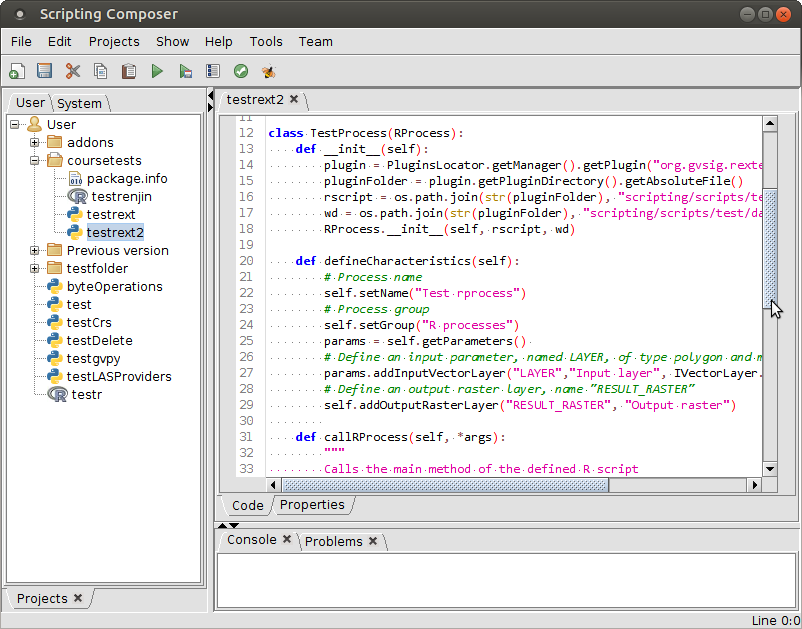
Have a closer look to each file. In gluecode.py we basically have: 1) some imports, a class declaration extending from RProcess class and an __init__ method defining the path to the rscript (and optionally the working directory):
import rlib
reload(rlib)
from rlib.process import *
import os

class TestProcess1(RProcess):
    def __init__(self):
        baseDir = os.path.dirname(os.path.abspath(__file__))
        rscript = os.path.join(baseDir, "rscript.r")
        RProcess.__init__(self, rscript, baseDir)
Exercise 3
Have a closer look to each file. In gluecode.py we basically have: 2) a defineCharacteristics method with the declaration of the inputs and outputs:
    def defineCharacteristics(self):
        # Process name
        self.setName("Test R process1")
        # Process group
        self.setGroup("Geostat course")
        params = self.getParameters()
        # Define an input vector parameter, named IN_VECTOR, of type polygon and make it mandatory
        params.addInputVectorLayer("IN_VECTOR","Input vector layer", SHAPE_TYPE_POLYGON, True)

        # Define an input raster parameter named IN_RASTER and make it mandatory
        params.addInputRasterLayer("IN_RASTER","Input raster layer", True)

        # Define an output raster layer, name "OUT_RASTER"
        self.addOutputRasterLayer("OUT_RASTER", "Output raster")
Exercise 3
Have a closer look to each file. In gluecode.py we basically have: 3) a callRProcess method defining the methods of the R script to be called:
    def callRProcess(self, *args):
        """
        Calls the main method of the defined R script
        """
        self.R.call("load_libraries")
        self.R.call("doalmostnothing", *args)
Exercise 3
- You could even omit callRProcess (then the main method of the R script would be called)
- You can also define more complex callRProcess methods if you want to somehow transform or reorder some parameters (see the examples on the provided sample scripts)
Exercise 3
Have a closer look to each file. In autorun.py script we instance the TestProcess1 that
we previously declared in gluecode.py and we register it on the toolbox:
import gvsig
from gluecode import *
import gluecode

process = gluecode.TestProcess1()
process.selfregister("Scripting")
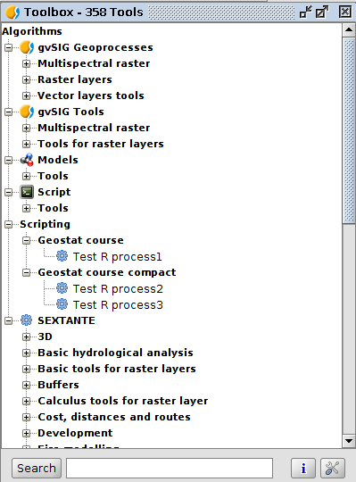
Exercise 3
This is enough to have the R plugin available on the gvSIG toolbox and process modeller
Exercise 2
Exercise 3
But we can do the same even with less code. Have a look to the geostatsplugincompact sample plugin. It only contains:
- The R script(s) to be integrated
- The autorun.py script, in which we do the declaration and registration of the R scripts altogether
- The empty __init__.py file
Exercise 3
If you look to autorun.py in geostatsplugincompact, you'll notice:
- We have omitted the __init__ method (we use self.rscript in defineCharacteristics instead
- We have also omitted the callRprocess method (because we have a main method in our R script)
Exercise 3
Now you are ready to integrate your own scripts. Follow these steps
- Open the gvSIG scripting composer (Tools -> Development -> Scripting composer)
- Create a new folder (File -> New), type the name (it will be the name of your plugin) and select Type: Folder
- Create the empty __init__.py script (File -> New), type: Script, language: Python, save on the folder you just created
Exercise 3
- Create the R script script (File -> New), type: Script, language: R. You can create it from scratch or you can paste an existing R script. You could also directly copy the file in the right folder, within ${HOME}/gvSIG/plugins/org.gvsig.scripting.app.mainplugin/scripts/yourpluginname
Exercise 3
- Finally, create the autorun.py script (File -> New), type: Script, language: Python
- You need to create a class per each R script you want to integrate
- IMPORTANT: the name of the class MUST be unique (even across different plugins)
- In each class, you need to declare:
- the path to the R script and its parameters (within the defineCharacteristics method)
- the R functions to call (within the callRProcess method)
- And you need to write the registration code at the end of the file (outside any class declaration)
Exercise 3
Once you test and validate your plugin, you are ready to distribute it. It's very easy!!
- From the Scripting Composer, click on menu Tools -> Script package
- Choose the folder you created (which contains all the scripts)
- Review the form details (name, version...)
- And finally select the output folder and file name
Exercise 3
This creates a .gvspkg file, which can be easily installed on other computer using gvSIG's Add-on Manager
You can also contact us to get your plugin included on the Standard installation list. In this way, your users will not need to download the package themselves
Exercise 3
